ADM1F_SRT: Input/output sensitivity¶

Here we explore the relationships between inputs and outputs. In the ADM1F: Execution time example we showed how to run the models with the perturbed input values from influent.dat and param.dat files. Assuming that you run the ADM1F: Execution time example and produced the outputs_influent.csv and outputs_params.csv files, we use these outputs here to study the relationship between influents and outputs, and params and outputs. If not just uncomment lines 5 and 18 and re-run the simulations.

Authors: Wenjuan Zhang and Elchin Jafarov

[1]:

import adm1f_utils as adm1fu
import os
import pandas as pd
import matplotlib.pyplot as plt
import seaborn as sns
%matplotlib inline

1. Influent/Output sensitivity¶

[2]:

# navigate to simulations folder
os.chdir('../../simulations')

[3]:

#Set the path to the ADM1F executable
ADM1F_EXE = '/Users/elchin/project/ADM1F_WM/build/adm1f'

# Set the value of percentage and sample size for lhs
percent = 0.1 # NOTE: for params percent should be <= 0.05
sample_size = 100
variable = 'influent'    # influent/params/ic
method = 'uniform'    #'uniform' or 'lhs'

[4]:

index=adm1fu.create_a_sample_matrix(variable,method,percent,sample_size)
print ()
print ('Number of elements participated in the sampling:',len(index))

Saves a sampling matrix [sample_size,array_size] into var_influent.csv
sample_size,array_size:  (100, 11)
Each column of the matrix corresponds to a variable perturbed 100 times around its original value
var_influent.csv SAVED!

Number of elements participated in the sampling: 11

[5]:

#exe_time=adm1fu.adm1f_output_sampling(ADM1F_EXE,variable,index)

[6]:

[output_name,output_unit]=adm1fu.get_output_names()
alloutputs = pd.read_csv('outputs_influent.csv', sep=',', header=None)
alloutputs.columns = output_name

[7]:

alloutputs

[7]:

	Ssu	Saa	Sfa	Sva	Sbu	Spro	Sac	Sh2	Sch4	Sic	...	Alk	NH3	NH4	LCFA	percentch4	energych4	efficiency	VFA/ALK	ACN	sampleT
0	7.37820	3.30795	56.7230	6.60272	8.46032	6.26942	1908.38	0.000123	48.7774	615.799	...	8148.98	8.64671	987.952	56.7230	57.2720	66.2091	52.7615	0.222004	116.5620	24.3594
1	7.28460	3.26614	55.8953	6.52078	8.34621	6.18289	2033.37	0.000121	48.4068	645.849	...	8602.48	9.61694	1048.750	55.8953	56.8728	65.9860	53.8907	0.223891	92.1431	24.8179
2	6.85866	3.07582	52.1661	6.11321	7.84990	5.79147	1926.30	0.000114	47.7048	651.060	...	8442.25	9.57599	1031.740	52.1661	56.7510	61.6157	52.8110	0.216106	125.4410	27.1630
3	6.72726	3.01709	51.0289	5.97094	7.70738	5.67153	1931.76	0.000112	47.6768	660.852	...	8558.31	9.84058	1044.000	51.0289	56.6698	61.9098	53.9655	0.213730	116.0810	27.9786
4	7.55763	3.38810	58.3212	6.83699	8.63179	6.43593	2242.26	0.000126	49.1049	657.957	...	9061.95	10.49270	1109.360	58.3212	57.2318	68.8331	51.4620	0.234238	77.3666	23.5162
...	...	...	...	...	...	...	...	...	...	...	...	...	...	...	...	...	...	...	...	...	...
95	7.65859	3.43319	59.2237	6.78604	8.84032	6.52986	1911.45	0.000128	48.9244	616.258	...	8197.36	8.37148	985.507	59.2237	56.5753	71.6467	52.7621	0.221140	125.5700	23.0752
96	7.40606	3.32040	56.9708	6.57190	8.52763	6.29525	2049.40	0.000123	48.6287	649.584	...	8699.15	9.58421	1054.650	56.9708	56.5357	69.7230	54.2485	0.223168	102.1390	24.2222
97	7.06582	3.16840	53.9710	6.30301	8.09601	5.98132	1778.88	0.000118	48.2397	605.950	...	7819.47	8.22490	949.405	53.9710	57.3804	61.6582	52.9718	0.215719	129.6520	25.9740
98	6.85456	3.07399	52.1312	6.12749	7.83407	5.78776	2146.27	0.000114	48.1629	685.484	...	9144.20	11.07250	1119.840	52.1312	56.8556	64.3136	53.8121	0.222069	88.1808	27.1834
99	7.44704	3.33870	57.3346	6.67541	8.53678	6.33321	1983.08	0.000124	48.5798	627.253	...	8349.28	9.04090	1016.750	57.3346	57.0513	66.1387	53.8114	0.225090	103.0960	24.0295

100 rows × 67 columns

[8]:

[influent_name,influent_index]=adm1fu.get_influent_names()

[9]:

# since we did not use all the columns in the influent.dat (see create_a_sample_matrix)
# we use index to select used headers for used values
header=[]
for i in index:
    header.append(influent_name[i])

influent_inputs = pd.read_csv('var_influent.csv', sep=',', header=None)
influent_inputs.columns = header
influent_inputs.head()

[9]:

	S_su_in	S_aa_in	S_fa_in	S_ac_in	S_IN_in	X_ch_biom_in	X_pr_biom_in	X_li_biom_in	X_I_in	Q	Temp
0	2.41679	4.54049	3.26551	1.06715	0.00794	8.21103	7.65897	5.45471	18.04704	139.57635	31.64409
1	2.71197	4.44197	2.94117	0.97991	0.00798	8.47247	8.44312	5.01331	16.95071	136.99766	32.47646
2	2.37594	4.05372	3.09329	1.10619	0.00801	8.84280	8.55680	4.62146	18.06979	125.17005	31.95536
3	2.70155	4.55292	3.31319	1.00561	0.00784	9.14260	8.30096	4.69829	17.67225	121.52161	37.86524
4	2.35939	4.30043	3.00319	1.05070	0.00860	8.26193	9.19056	5.36216	19.24420	144.58137	35.68530

[10]:

# merge influent and output datasets
inout=pd.concat([influent_inputs,alloutputs], axis=1)
inout.head()

[10]:

	S_su_in	S_aa_in	S_fa_in	S_ac_in	S_IN_in	X_ch_biom_in	X_pr_biom_in	X_li_biom_in	X_I_in	Q	...	Alk	NH3	NH4	LCFA	percentch4	energych4	efficiency	VFA/ALK	ACN	sampleT
0	2.41679	4.54049	3.26551	1.06715	0.00794	8.21103	7.65897	5.45471	18.04704	139.57635	...	8148.98	8.64671	987.952	56.7230	57.2720	66.2091	52.7615	0.222004	116.5620	24.3594
1	2.71197	4.44197	2.94117	0.97991	0.00798	8.47247	8.44312	5.01331	16.95071	136.99766	...	8602.48	9.61694	1048.750	55.8953	56.8728	65.9860	53.8907	0.223891	92.1431	24.8179
2	2.37594	4.05372	3.09329	1.10619	0.00801	8.84280	8.55680	4.62146	18.06979	125.17005	...	8442.25	9.57599	1031.740	52.1661	56.7510	61.6157	52.8110	0.216106	125.4410	27.1630
3	2.70155	4.55292	3.31319	1.00561	0.00784	9.14260	8.30096	4.69829	17.67225	121.52161	...	8558.31	9.84058	1044.000	51.0289	56.6698	61.9098	53.9655	0.213730	116.0810	27.9786
4	2.35939	4.30043	3.00319	1.05070	0.00860	8.26193	9.19056	5.36216	19.24420	144.58137	...	9061.95	10.49270	1109.360	58.3212	57.2318	68.8331	51.4620	0.234238	77.3666	23.5162

5 rows × 78 columns

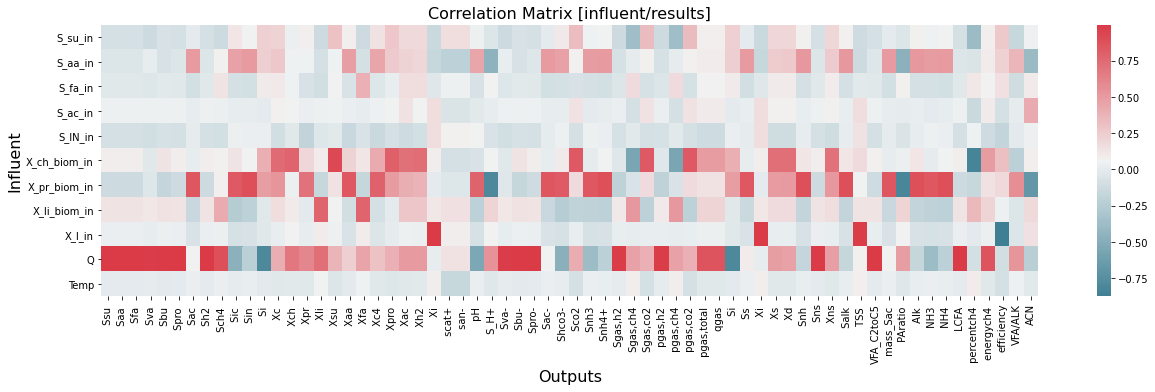
The correlation heat map matrix below shows that four influents have the highest impact on the results: X_ch_biom_in, X_pr_biom_in, X_li_biom_in, and Q.

[11]:

corr=inout.corr()
plt.figure(figsize=(21,5))
sns.heatmap(corr.iloc[0:11,11:-1], cmap=sns.diverging_palette(220, 10, as_cmap=True))
plt.title('Correlation Matrix [influent/results]',fontsize=16);
plt.ylabel('Influent',fontsize=16)
plt.xlabel('Outputs',fontsize=16)

[11]:

Text(0.5, 23.09375, 'Outputs')

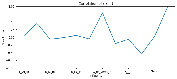
../_images/jupyter_notebook_io_sensitivity_analysis_13_1.png

Let’s merge ph values from the results with the influents and explore the correlations.

[12]:

influent_ph=pd.concat([influent_inputs,alloutputs[' pH ']], axis=1)

[13]:

plt.figure(figsize=(10,4))
influent_ph.corr().iloc[-1].plot(linewidth=2)
plt.title('Correlation plot (ph)')
plt.xlabel('Influents')
plt.ylabel('Correlation')
plt.ylim([-1,1])

[13]:

(-1.0, 1.0)

../_images/jupyter_notebook_io_sensitivity_analysis_16_1.png

[14]:

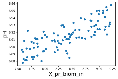
plt.scatter( influent_ph['X_pr_biom_in'],influent_ph[' pH '])
plt.xlabel('X_pr_biom_in',fontsize=18)
plt.ylabel('pH',fontsize=18);

../_images/jupyter_notebook_io_sensitivity_analysis_17_0.png

[15]:

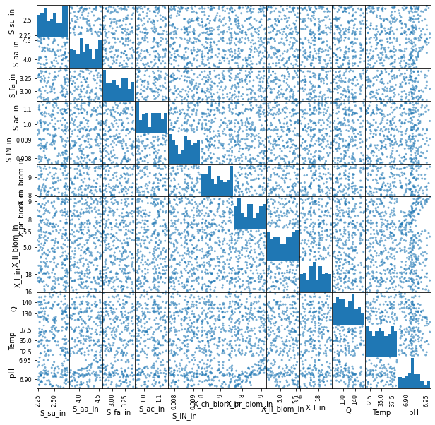
from pandas.plotting import scatter_matrix
scatter_matrix(influent_ph, alpha=0.6,figsize=(10,10));

../_images/jupyter_notebook_io_sensitivity_analysis_18_0.png

2. Params/Output sensitivity¶

[16]:

# Set the value of percentage and sample size for lhs
percent = 0.1 # NOTE: for params percent should be <= 0.05
sample_size = 100
variable = 'params'    # influent/params/ic
method = 'uniform'    #'uniform' or 'lhs'

[17]:

index=adm1fu.create_a_sample_matrix(variable,method,percent,sample_size)
print ()
print ('Number of elements participated in the sampling:',len(index))

Saves a sampling matrix [sample_size,array_size] into var_params.csv
sample_size,array_size:  (100, 92)
Each column of the matrix corresponds to a variable perturbed 100 times around its original value
var_params.csv SAVED!

Number of elements participated in the sampling: 92

[18]:

#exe_time=adm1fu.adm1f_output_sampling(ADM1F_EXE,variable,index)

[19]:

[output_name,output_unit]=adm1fu.get_output_names()
alloutputs = pd.read_csv('outputs_params.csv', sep=',', header=None)
alloutputs.columns = output_name

[20]:

[param_name,param_index]=adm1fu.get_param_names()

[21]:

# since we did not use all the columns in the influent.dat (see create_a_sample_matrix)
# we use index to select used headers for used values
header=[]
for i in index:
    header.append(param_name[i])

param_inputs = pd.read_csv('var_params.csv', sep=',', header=None)
param_inputs.columns = header
param_inputs.head()

[21]:

	f_sI_xc	f_xI_xc	f_ch_xc	f_pr_xc	f_li_xc	N_xc	N_I	N_aa	C_xc	C_sI	...	k_A_Bpro	k_A_Bac	k_A_Bco2	k_A_BIN	kLa	K_H_h2o_base	K_H_co2_base	K_H_ch4_base	K_H_h2_base	k_P
0	0.09116	0.27346	0.21535	0.21711	0.27475	0.00251	0.00420	0.00736	0.02895	0.02792	...	1.026524e+10	1.086406e+10	9.205019e+09	1.087446e+10	207.51543	0.02859	0.03361	0.00146	0.00071	50821.70460
1	0.09692	0.25605	0.18183	0.21486	0.27367	0.00293	0.00450	0.00648	0.02930	0.02715	...	9.961014e+09	9.209860e+09	9.484090e+09	1.097333e+10	185.69982	0.03129	0.03583	0.00146	0.00079	45097.70847
2	0.09653	0.25089	0.18351	0.19403	0.22666	0.00246	0.00420	0.00649	0.02824	0.03114	...	1.043165e+10	1.081807e+10	9.359366e+09	9.475087e+09	218.85580	0.02930	0.03748	0.00140	0.00074	53707.49901
3	0.09891	0.25074	0.19437	0.20372	0.23318	0.00263	0.00468	0.00666	0.02873	0.02895	...	9.431350e+09	1.031777e+10	9.787729e+09	1.030247e+10	184.26372	0.03229	0.03850	0.00127	0.00086	49069.07961
4	0.10742	0.26412	0.20268	0.20954	0.26893	0.00263	0.00414	0.00723	0.02958	0.03157	...	1.090281e+10	1.020322e+10	1.063838e+10	1.076841e+10	189.12319	0.02950	0.03578	0.00138	0.00083	54000.23123

5 rows × 92 columns

[22]:

# merge influent and output datasets
inout=pd.concat([param_inputs,alloutputs], axis=1)
inout.head()

[22]:

	f_sI_xc	f_xI_xc	f_ch_xc	f_pr_xc	f_li_xc	N_xc	N_I	N_aa	C_xc	C_sI	...	Alk	NH3	NH4	LCFA	percentch4	energych4	efficiency	VFA/ALK	ACN	sampleT
0	0.09116	0.27346	0.21535	0.21711	0.27475	0.00251	0.00420	0.00736	0.02895	0.02792	...	8909.63	9.53919	1060.990	61.5561	56.0945	65.7436	52.8869	0.222452	87.1484	25.3731
1	0.09692	0.25605	0.18183	0.21486	0.27367	0.00293	0.00450	0.00648	0.02930	0.02715	...	7707.69	10.88420	927.238	56.1139	62.1148	62.3272	55.0303	0.147138	654.5290	25.3731
2	0.09653	0.25089	0.18351	0.19403	0.22666	0.00246	0.00420	0.00649	0.02824	0.03114	...	7873.10	8.67396	927.390	68.2248	58.8253	64.9817	54.1026	0.191081	196.3670	25.3731
3	0.09891	0.25074	0.19437	0.20372	0.23318	0.00263	0.00468	0.00666	0.02873	0.02895	...	7961.45	10.83540	953.650	64.3854	57.4965	66.4942	55.2003	0.118815	-1663.6400	25.3731
4	0.10742	0.26412	0.20268	0.20954	0.26893	0.00263	0.00414	0.00723	0.02958	0.03157	...	8755.37	10.43910	1081.950	67.7978	56.9557	64.9350	53.1639	0.222974	94.6821	25.3731

5 rows × 159 columns

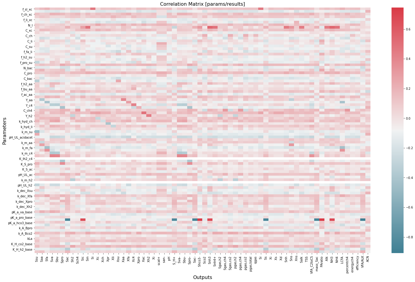
[23]:

corr=inout.corr()
plt.figure(figsize=(25,15))
sns.heatmap(corr.iloc[0:92,92:-1], cmap=sns.diverging_palette(220, 10, as_cmap=True))
plt.title('Correlation Matrix [params/results]',fontsize=16);
plt.ylabel('Parameters',fontsize=16)
plt.xlabel('Outputs',fontsize=16)

[23]:

Text(0.5, 113.09375, 'Outputs')

../_images/jupyter_notebook_io_sensitivity_analysis_27_1.png

[ ]: