ADM1F SRT: single tank and two-phase anaerobic dynamic membrane bioreactor¶

This script is used to simulate a single tank suspended anaerobic dynamic membrane digester and a novel two-phase anaerobic dynamic membrane bioreator with separated SRT and HRT. In the two-phase reactor the effluent (model output) from the first phase dynamic membrane bioreactor is converted to the influent (model input) for the second-phase anaerobic dynamic membrane bioreactor as shown in the figure.

Note: Before running the ADM1F SRT simulations see intructions on how to compile adm1f_srt.cxx in the User Guide.

Mass balance equation with SRT:

The ADM1 and ADM1F solve the mass balance equation (i.e. mass_change = mass_in – mass_out + reaction). ADM1F_SRT version of the model includes solid retention time (\(t_{res,X}\)) as shown in the equation below.

\[\frac{d\, S_{\text{liq,i}}}{dt} = \frac{qS_{\text{in,i}}}{V_{\text{liq}}} - \frac{qS_{\text{liq,i}} }{V_{\text{liq}}}+ \sum_{j=1}^{12}\rho_{j} v_{i,j}\]

\[\frac{d\, X_{\text{liq,i}}}{dt} = \frac{qX_{\text{in,i}}}{V_{\text{liq}}} - \frac{X_{\text{liq,i}}}{t_{\text{res,X}} + V_{\text{liq}}/q} + \sum_{j=13}^{24}\rho_{j} v_{i,j}\]

Authors: Wenjuan Zhang, Elchin Jafarov, Kuang Zhu

[1]:

# Load packages
import numpy as np
import pandas as pd
import os
import seaborn as sns
import adm1f_utils as adm1fu
import matplotlib.pyplot as plt
%matplotlib inline

[2]:

# navigate to simulations folder
os.chdir('../simulations')

[3]:

# Grab the names and unit of all the outputs
(output_name,output_unit)=adm1fu.get_output_names()

[4]:

#check the path to the executable
!echo $ADM1F_EXE

/Users/elchin/project/ADM1F_WM/build/adm1f

Single tank anaerobic dynamic membrane bioreactor (AnDMBR)¶

To simulate the single tank AnDMBR that has separated SRT and HRT, We can call the functionreactor1 with different Q (flow-rate), Vliq (reactor volume), t_resx (SRT-HRT) values, the function will return the corresponding output

Usage example: reactor1(Q=100, t_resx=30, Vliq=300)

(Unit) Q: [m3/d], t_resx: [day], Vliq: [m3]

[5]:

# testing different SRTs=[0,1,2,...9] on the one-phase reactor
resx_list = [i for i in range(10)]
# setup the matrix with columns correspoding SRTs and rows to outputs
output1_resx = np.zeros((len(resx_list), 67))
# here we utilize back euler solver and adataptive time step
# for more command options see "User Guide/Running ADM1F/step 5"
options='-ts_type beuler -ts_adapt_type basic -ts_max_snes_failures -1 -steady'

for i in range(len(resx_list)):
    output1_resx[i] = adm1fu.reactor1(opt=options, Vliq=300, Q=600, t_resx=resx_list[i])

np.savetxt('output_1phase.csv',output1_resx,delimiter=',',fmt='%1.4e')

Reactor run, phase-one:
$ADM1F_EXE -ts_type beuler -ts_adapt_type basic -ts_max_snes_failures -1 -steady -Vliq 300 -t_resx 0 -influent_file influent_cur.dat
indicator-228.out
Reactor run, phase-one:
$ADM1F_EXE -ts_type beuler -ts_adapt_type basic -ts_max_snes_failures -1 -steady -Vliq 300 -t_resx 1 -influent_file influent_cur.dat
indicator-307.out
Reactor run, phase-one:
$ADM1F_EXE -ts_type beuler -ts_adapt_type basic -ts_max_snes_failures -1 -steady -Vliq 300 -t_resx 2 -influent_file influent_cur.dat
indicator-437.out
Reactor run, phase-one:
$ADM1F_EXE -ts_type beuler -ts_adapt_type basic -ts_max_snes_failures -1 -steady -Vliq 300 -t_resx 3 -influent_file influent_cur.dat
indicator-563.out
Reactor run, phase-one:
$ADM1F_EXE -ts_type beuler -ts_adapt_type basic -ts_max_snes_failures -1 -steady -Vliq 300 -t_resx 4 -influent_file influent_cur.dat
indicator-521.out
Reactor run, phase-one:
$ADM1F_EXE -ts_type beuler -ts_adapt_type basic -ts_max_snes_failures -1 -steady -Vliq 300 -t_resx 5 -influent_file influent_cur.dat
indicator-516.out
Reactor run, phase-one:
$ADM1F_EXE -ts_type beuler -ts_adapt_type basic -ts_max_snes_failures -1 -steady -Vliq 300 -t_resx 6 -influent_file influent_cur.dat
indicator-534.out
Reactor run, phase-one:
$ADM1F_EXE -ts_type beuler -ts_adapt_type basic -ts_max_snes_failures -1 -steady -Vliq 300 -t_resx 7 -influent_file influent_cur.dat
indicator-542.out
Reactor run, phase-one:
$ADM1F_EXE -ts_type beuler -ts_adapt_type basic -ts_max_snes_failures -1 -steady -Vliq 300 -t_resx 8 -influent_file influent_cur.dat
indicator-556.out
Reactor run, phase-one:
$ADM1F_EXE -ts_type beuler -ts_adapt_type basic -ts_max_snes_failures -1 -steady -Vliq 300 -t_resx 9 -influent_file influent_cur.dat
indicator-576.out

[6]:

df1_resx = pd.read_csv('output_1phase.csv', sep=',', header=None)
df1_resx.columns = output_name
df1_resx.insert(0,"T_resx",resx_list)

Relation between t_resx and output when Vliq=300m3, Q=600m3/d

[7]:

# check the results with increasing T_resx, we should expect decrease in Ssu
df1_resx

[7]:

	T_resx	Ssu	Saa	Sfa	Sva	Sbu	Spro	Sac	Sh2	Sch4	...	Alk	NH3	NH4	LCFA	percentch4	energych4	efficiency	VFA/ALK	ACN	sampleT
0	0	2152.800	324.2700	7382.70	2381.700	3667.300	2542.700	8263.5	25.643000	-8.963700e-82	...	44957.0	0.053067	1074.00	7382.70	-1.133000e-81	83.808	3.9774	0.351490	-3.203400e-72	0.5
1	1	123.060	49.1670	7751.20	2574.400	4202.900	3244.500	9600.7	30.352000	3.859800e-12	...	59182.0	0.047701	1135.60	7751.20	1.599000e-12	100.630	-76.4800	0.310840	1.255000e-08	0.5
2	2	63.057	26.6380	7839.00	2610.000	4268.600	3305.000	9742.9	30.772000	1.085400e-09	...	61421.0	0.048208	1150.90	7839.00	4.422100e-10	102.210	-155.0200	0.304150	2.777100e-07	0.5
3	3	39.313	17.3450	908.19	41.129	54.118	53.411	3339.7	0.000662	2.574900e+02	...	16289.0	2.513100	963.03	908.19	5.579800e+01	209.370	-218.4400	0.200760	9.097200e+00	0.5
4	4	30.634	13.5750	457.20	30.592	39.989	35.895	3066.6	0.000515	2.653300e+02	...	18846.0	3.157300	963.70	457.20	5.623900e+01	214.510	-304.2100	0.157850	1.324200e+01	0.5
5	5	25.261	11.2240	309.54	24.543	31.958	27.254	2856.4	0.000424	2.695900e+02	...	21319.0	3.693200	966.73	309.54	5.648800e+01	217.230	-390.0200	0.129290	1.778600e+01	0.5
6	6	21.606	9.6181	236.08	20.615	26.775	22.111	2685.8	0.000362	2.726300e+02	...	23721.0	4.147900	970.17	236.08	5.666900e+01	219.140	-475.6200	0.108900	2.279000e+01	0.5
7	7	18.960	8.4513	192.14	17.859	23.153	18.702	2543.7	0.000317	2.750200e+02	...	26050.0	4.540600	973.69	192.14	5.681200e+01	220.630	-560.8900	0.093693	2.825000e+01	0.5
8	8	16.955	7.5652	162.87	15.818	20.479	16.276	2423.2	0.000284	2.770000e+02	...	28311.0	4.885500	977.21	162.87	5.692900e+01	221.870	-645.8400	0.081984	3.416600e+01	0.5
9	9	15.383	6.8691	141.96	14.244	18.422	14.462	2319.3	0.000257	2.786900e+02	...	30505.0	5.192300	980.68	141.96	5.702800e+01	222.920	-730.4900	0.072728	4.053400e+01	0.5

10 rows × 68 columns

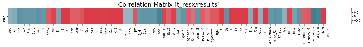
[8]:

# correlation between SRT and output
plt.figure(figsize=(24,1))
corr1=df1_resx.corr()
sns.heatmap(corr1.iloc[0:1,-67:], xticklabels=df1_resx.columns[-67:], yticklabels=df1_resx.columns[0:1], cmap=sns.diverging_palette(220, 10, as_cmap=True))
plt.title('Correlation Matrix [t_resx/results]',fontsize=20);

../_images/jupyter_notebook_ADM1F_SRT_2phase_11_0.png

Configurations

Configuration	Vliq (m\(^3\))	t_resx (d)	Q (m\(^3\)/d)
Default	3400	0	134
Phase 1	340	1.5	618
Phase 2	3400	700	618/—

where t_resx = SRT - HRT

[9]:

config_default = {'Vliq':3400, 't_resx':0, 'Q':134}
config1 = {'Vliq':340, 't_resx':1.5, 'Q':618}
config2 = {'Vliq':3400, 't_resx':700, 'Q':618}

Default Configuration¶

[10]:

# output using default configuration
ls_default = adm1fu.reactor1(**config_default).tolist()
df_default = pd.DataFrame(data = [ls_default],columns=output_name, index=['Default Configuration'])
df_default

Reactor run, phase-one:
$ADM1F_EXE  -Vliq 3400 -t_resx 0 -influent_file influent_cur.dat
indicator-034.out

[10]:

	Ssu	Saa	Sfa	Sva	Sbu	Spro	Sac	Sh2	Sch4	Sic	...	Alk	NH3	NH4	LCFA	percentch4	energych4	efficiency	VFA/ALK	ACN	sampleT
Default Configuration	7.17674	3.21796	54.9446	6.39778	8.23228	6.08339	1963.6	0.00012	48.3303	639.764	...	8438.52	9.32395	1026.69	54.9446	56.905	65.228	53.3712	0.220453	109.164	25.3731

1 rows × 67 columns

Configuration 1¶

[11]:

# output using configuration 1
ls_config1 = adm1fu.reactor1(**config1).tolist()
df_config1 = pd.DataFrame(data = [ls_config1],columns=output_name, index=['Phase 1 Configuration'])
df_config1

Reactor run, phase-one:
$ADM1F_EXE  -Vliq 340 -t_resx 1.5 -influent_file influent_cur.dat
indicator-051.out

[11]:

	Ssu	Saa	Sfa	Sva	Sbu	Spro	Sac	Sh2	Sch4	Sic	...	Alk	NH3	NH4	LCFA	percentch4	energych4	efficiency	VFA/ALK	ACN	sampleT
Phase 1 Configuration	80.5616	33.4704	7808.75	2598.14	4246.87	3285.25	9696.05	28.5069	7.737870e-30	147.214	...	60316.4	0.048011	1145.6	7808.75	3.164870e-30	104.203	-104.737	0.308161	1.202840e-17	0.550162

1 rows × 67 columns

Configuration 2¶

[12]:

# output using configuration 2
ls_config2 = adm1fu.reactor1(**config2).tolist()
df_config2 = pd.DataFrame(data = [ls_config2],columns=output_name, index=['Phase 2 Configuration'])
df_config2

Reactor run, phase-one:
$ADM1F_EXE  -Vliq 3400 -t_resx 700 -influent_file influent_cur.dat
indicator-025.out

[12]:

	Ssu	Saa	Sfa	Sva	Sbu	Spro	Sac	Sh2	Sch4	Sic	...	Alk	NH3	NH4	LCFA	percentch4	energych4	efficiency	VFA/ALK	ACN	sampleT
Phase 2 Configuration	2.70068	1.20723	19.0168	2.34856	3.01652	2.16597	1125.18	0.000045	75.1774	952.376	...	21574.7	14.7549	1186.64	19.0168	58.194	255.569	-899.833	0.049221	3302.96	5.50162

1 rows × 67 columns

Two-Phase anaerobic dynamic membrane bioreactor¶

To simulate a novel two-phase AnDMBR, We can call the function reactor2 with different Q1 (phase 1 flow rate), Q2 (phase 2 flow rate, normally equal to Q1), Vliq1 (phase 1 volume), Vliq2 (phase 2 volume), t_resx1 (SRT-HRT for phase 1), and t_resx2 (SRT-HRT for phase 1) values. In this function, the model output from phase 1 will be extracted and converted to the model input for phase 2. The function will return phase1 output and phase2 output

Usage example: reactor2(Q1=100, t_resx1=30, t_resx2=100, Vliq1=300, Vliq2=3000)

[13]:

from IPython.display import Image
print ('Schematics of the two-phase reactor')
Image(filename='../notebooks/2phase_reactor.png')

Schematics of the two-phase reactor

[13]:

../_images/jupyter_notebook_ADM1F_SRT_2phase_21_1.png

Config12¶

Configurations

Configuration	Vliq (m\(^3\))	t_resx (d)	Q (m\(^3\)/d)
Default	3400	0	134
Phase 1	340	1.5	618
Phase 2	3400	700	618/—

where t_resx = SRT - HRT

[14]:

# config12 = {"Vliq1":340, "Vliq2":3400, "t_resx1":1.5, "t_resx2":700, "Q1":618, "Q2":618}
config12 = {"Vliq1":340, "Vliq2":3400, "t_resx1":1.5, "t_resx2":700, "Q1":618}

[15]:

result_config12 = adm1fu.reactor2(**config12)

Reactor run, phase-one:
$ADM1F_EXE  -Vliq 340 -t_resx 1.5 -influent_file influent_cur.dat
indicator-051.out
Reactor run, phase-two:
$ADM1F_EXE -Vliq 3400 -t_resx 700 -influent_file influent_cur.dat
indicator-024.out

[16]:

# output using config12
result_config12 = adm1fu.reactor2(**config12)
ls1_config12 = result_config12[0].tolist()
ls2_config12 = result_config12[1].tolist()

df_config12 = pd.DataFrame(data = [ls1_config12],columns=output_name,index=['Phase1'])
df_config12.loc['Phase2'] = ls2_config12
df_config12

Reactor run, phase-one:
$ADM1F_EXE  -Vliq 340 -t_resx 1.5 -influent_file influent_cur.dat
indicator-051.out
Reactor run, phase-two:
$ADM1F_EXE -Vliq 3400 -t_resx 700 -influent_file influent_cur.dat
indicator-024.out

[16]:

	Ssu	Saa	Sfa	Sva	Sbu	Spro	Sac	Sh2	Sch4	Sic	...	Alk	NH3	NH4	LCFA	percentch4	energych4	efficiency	VFA/ALK	ACN	sampleT
Phase1	80.561600	33.470400	7808.7500	2598.14000	4246.87000	3285.25000	9696.05	28.506900	7.771710e-32	147.214	...	60316.4	0.048011	1145.6	7808.7500	3.068330e-32	104.203	-104.737	0.308161	1.216580e-18	0.550162
Phase2	0.355681	0.132504	19.2757	2.37729	3.05196	2.19399	1248.96	0.000046	7.114040e+01	867.356	...	17101.8	15.289200	1139.4	19.2757	6.198330e+01	192.277	-590.307	0.068884	-2.807000e+01	6.241160

2 rows × 67 columns

[ ]: